2.7. Scientific diagnostics
Warning
These functions work, at this time, only for z-coordinate models (NEMO for instance). But they can provide some ideas on diagnostics.
2.7.1. Section transports
The pypago.secdiag module contains several functions to compute transport across gridded sections.
Note
The total tracer transport must be equal to overturning + barotropic + baroclinic tracer transports: TOT = OVT + BAR + BC
A complete example of transport calculations is shown below:
import pypago.pyio
import pypago.misc
import pypago.secdiag as diag
import pylab as plt
import numpy as np
from pypago.sample_param import rho0_c

# loading section data
sections = pypago.pyio.load('data/indian_datasec.pygo')

# extraction of the "section4" section
indsec = pypago.misc.findsecnum(sections, 'section4')
sec = sections[indsec]

# creation of xticklabels
index = np.arange(0, len(sec.time_counter))
xlabels = np.array([d.strftime('%Y-%m-%d') for d in sec.time_counter])

# calculation of net volume transport
netvt = diag.net_volume_trans(sec, velname='vel') * 1e-6

# calculation of net heat transport
netht = diag.net_tracer_trans(sec, 'temp', velname='vel') * 1e-15 * rho0_c

# calculation of velocity without net transport
current_nonet = diag.remove_spatial_mean(sec, 'vel')

# calculation of total heat transport (i.e. without net mass transport)
totht = diag.total_tracer_trans(sec, 'temp', 'vel') * 1e-15 * rho0_c

# calculation of temperature anomalies
temp_nonet = diag.remove_spatial_mean(sec, 'temp')

# overturning volume transport
ovvt = diag.overturning_volume_transport(sec, 'vel')

# overturning heat transport
ovht = diag.overturning_tracer_transport(sec, 'temp', 'vel') * 1e-15 * rho0_c

# barotropic volume transport
barvt = diag.barotropic_volume_transport(sec, 'vel')

# barotropic heat transport
barht = diag.barotropic_tracer_transport(sec, 'temp', 'vel') * 1e-15 * rho0_c

# baroclinic heat transport
bcht = diag.baroclinic_tracer_transport(sec, 'temp', 'vel') * 1e-15 * rho0_c

plt.figure()
plt.subplots_adjust(left=0.1, right=0.99,
                    top=0.95, bottom=0.05, hspace=0.25)

plt.subplot(2, 2, 1)
plt.plot(totht, label='totht')
plt.plot(ovht + barht + bcht, label='sum')
plt.title('totht')
plt.legend()

plt.subplot(2, 2, 2)
plt.plot(ovht)
plt.title('ovht')

plt.subplot(2, 2, 3)
plt.plot(barht)
plt.title('barht')

plt.subplot(2, 2, 4)
plt.plot(bcht)
plt.title('bcht')

plt.savefig('figs/heat_transport.png')
In [1]: import os

In [2]: cwd = os.getcwd()

In [3]: print(cwd)
/home/barrier/Codes/pago/pypago/doc_pypago

In [4]: fpath = "examples/section_transport.py"

In [5]: with open(fpath) as f:
   ...:     code = compile(f.read(), fpath, 'exec')
   ...:     exec(code)
   ...:
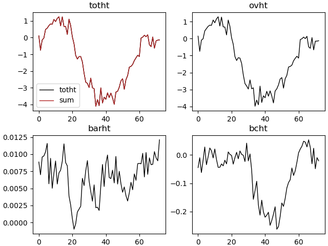
Fig. 2.23 Example of heat transport calculations.
2.7.2. Volume/Surface integration over domains
The pypago.areadiag module contains several functions in order to perform volume and surface integrations. These functions can be used for instance to tracer budgets calculations
over closed domains
In the example below, a heat budget calculation is performed over a closed domain, as in [BDTC15]. It is based on the following equations:
with \(\rho_0\) and \(C_p\) the reference density and heat capacity of sea-water, \(T\) the three-dimensional temperature, \(S_a\) the surface of the water volume \(V\) that is in contact with the atmosphere, \(SST\) and \(\eta\) the sea-surface temperature and sea-surface height.with \(\rho_0\) and \(C_p\) the reference density and heat capacity of sea-water, \(T\) the three-dimensional temperature, \(S_a\) the surface of the water volume \(V\) that is in contact with the atmosphere, \(SST\) and \(\eta\) the sea-surface temperature and sea-surface height.
with \(Q_{net}\) the net (latent, sensible, shortwave and longwave) surface heat fluxes, \(S_o\) the outline surface of volume \(V\) and \([UT]\) the ocean heat transport. The first term on the right-hand side of equation (2.2) represents the contribution of surface heat fluxes to changes in ocean heat content. In the following, a positive contribution implies that the ocean is warmed by the atmosphere (i.e. surface heat fluxes are, by convention, positive downwardwith \(Q_{net}\) the net (latent, sensible, shortwave and longwave) surface heat fluxes, \(S_o\) the outline surface of volume \(V\) and \([UT]\) the ocean heat transport. The first term on the right-hand side of equation (2.2) represents the contribution of surface heat fluxes to changes in ocean heat content. In the following, a positive contribution implies that the ocean is warmed by the atmosphere (i.e. surface heat fluxes are, by convention, positive downward)
import pypago.pyio
import pypago.misc
import pypago.secdiag as secdiag
import pypago.areadiag as areadiag
import pylab as plt
import numpy as np
from pypago.sample_param import rho0_c

data = pypago.pyio.load('data/natl_datadom.pygo')
area = data[0]

# calculation of the SSH * SSH product within the area
# and adding it to the area structure
area.surfhc = area.temp[:, 0, :] * area.ssh

# calculation of domain heat content
hc = areadiag.volume_content(area, 'temp')

# calculation of surface integral of SST * SSH
surfhc = areadiag.surface_content(area, 'surfhc')

# adding the surface heat content to the total heat content
hc += surfhc

# calculation of surface heat flux
hf = areadiag.surface_content(area, 'hf')

# loading of the gridded section domain
sections = pypago.pyio.load('data/natl_datasec.pygo')

# computation of heat convergence
heatconv = areadiag.compute_tracer_conv(area, sections, 'temp', 'vel')

# Conversion of hc and heat conv into J and W, respectively
hc *= rho0_c   # J
heatconv *= rho0_c    # W

# calculation of dt and conversion into seconds
dt = area.time_counter[1:] - area.time_counter[0:-1]
dt = np.array([d.total_seconds() for d in dt])

# time derivative of ocean heat content
dhc = np.diff(hc) / dt

# averaging of heat convergence and heat flux
# to fit the location of hc
heatconv = 0.5*(heatconv[1:] + heatconv[:-1])
hf = 0.5*(hf[1:] + hf[:-1])

# conversion from W into PW
hf *= 1e-15
dhc *= 1e-15
heatconv *= 1e-15

# Plotting
plt.figure()
ax1 = plt.gca()
plt.plot(dhc, label=r'$\partial hc  / \partial t$')
plt.plot(hf, label='$H_{flux}$')
plt.plot(heatconv + hf, label='$H_{flux} + H_{conv}$')
plt.legend(loc=8)
ax1.set_ylabel('(PW)')
ax2 = ax1.twinx()
plt.plot(heatconv, label='$H_{conv}$', color='plum')
plt.xlim(0, len(hf)-1)
ax2.set_ylabel(r'$H_{conv}$' + ' (PW)', color='plum')
plt.setp(ax2.get_yticklabels(), color='plum')
plt.savefig('figs/heat_budget.png')
In [6]: import os

In [7]: cwd = os.getcwd()

In [8]: print(cwd)
/home/barrier/Codes/pago/pypago/doc_pypago

In [9]: fpath = "examples/area_diags.py"

In [10]: with open(fpath) as f:
   ....:     code = compile(f.read(), fpath, 'exec')
   ....:     exec(code)
   ....:
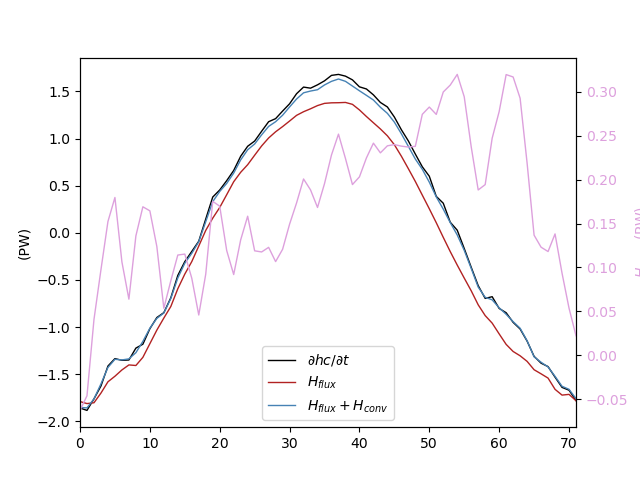
Fig. 2.24 Example of heat transport calculations.